TMG parameter computation

(A case study in practical use of elementary numerical methods)

Synopsis

This article shows how elementary numerical methods (e.g. Lagrange interpolation, computation of zeros, numerical differentiation) can be used to produce useful real-world results. As a case study, I will show the algorithms used to analyze muscle contraction speed in tensiomyography (TMG) measurements.

I spent my first few years out of university working with TMG BMC d.o.o., a Slovene company that invented and produces tensiomyography measurement systems.

[Link to TMG Wikipedia]

Clients of TMG are typically interested in the contraction speed and characteristics of a muscle. We quantify a muscle's contraction properties by computing 5 descriptive parameters from each TMG measurement. This article walks through the numerical techniques used in the computation of these parameters.

For context, here is a 10-second video of what a TMG measurement looks like:

[TODO]

To summarize the video: an electrical stimulus induces an involuntary muscle contraction, causing the surface of the muscle to rise and fall as the muscle contracts and relaxes. A displacement sensor placed against the muscle perpendicular to the muscle surface tracks the rise and fall of the muscle by sampling the muscle belly's displacement over time at 1 kHz.

The result is a displacement-time graph tracking the rise and fall of the muscle belly as the muscle contracts and then relaxes under electrical stimulus.

A typical response looks something like this:

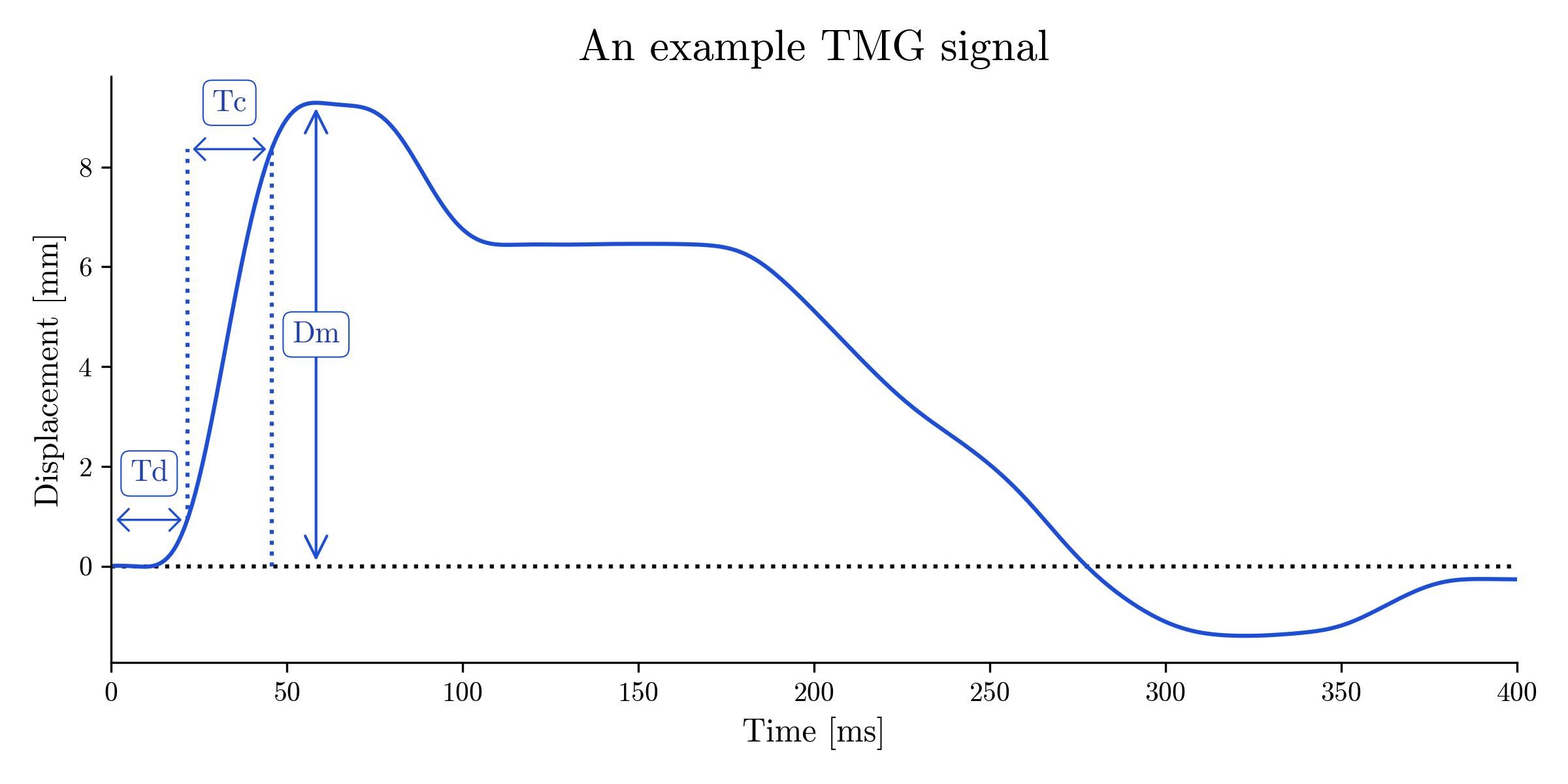
Plot of a typical TMG signal showing the rise and fall of a muscle as it contracts and relaxes under electrical stimulus. The parameters Dm, Td, and Tc characterise the amplitude and speed of muscle contraction.

You will note 5 parameters marked on the graph. These are:

Name	Abbreviation	Definition
Maximum displacement	Dm	Maximum amplitude of muscle contraction*
Delay time	Td	The time from the start of the TMG signal to the point at which the TMG signal first reaches 10 percent of its maximum value.
Contraction time	Tc	The time from the point at which the TMG signal first reaches 10 percent of its maximum value to the point at which the TMG signal first reaches 90 percent of its maximum value. (Analogous to the rise time parameter used in electronics to quantify the rise time of a pulse.)
Sustain time	Ts	The time the TMG signal remains above 50 percent of its maximum value.
Relaxation time	Tr	The time from the point at which the TMG signal has decayed to 90 percent of its maximum value to the point at which the TMG signal decays to 50 percent of its maximum value.

*subject to a few caveats that make determining maximum amplitude a little less trivial than it sounds.

Practical applications

Dm, Td, and Tc are indicative of speed and power.

Empirically, we have found that

Trained sprinters, for example, will have consistently faster values of Tc and Td, and larger values of Dm, than non-explosive athletes.

One can use TMG parameters to monitor effectiveness of a training program: if contraction speeds increase, the program is effectively developing speed and power (the athlete is improving recruitment of fast-twitch muscle fibers).

Conversely, TMG parameters are useful for injury detection and management. An athlete's contraction times fall below baseline levels after an injury. When values return to baseline, the muscle has physiologically recovered, and the athlete is ready to return to play.

Similarly, contraction times below baseline indicate muscle damage and suggest rest/recovery is appropriate, even if a macroscopic injury is not shown up (yet).

And asymmetries in contraction time and magnitude between left/right muscles imply injury risk, and suggest a training program to balance these asymmetries.

Ts and Tr are included for research reasons.

On the computational side, my goal is to take the TMG measurement as input and use it to compute the 5 characteristic parameters. A precise problem statement follows below.

Problem statement

Given a TMG measurement of a muscle's displacement over time under electrical stimulus (in practice recorded using a TMG S2 measurement system at 1 kHz sampling for 1000 ms for a total of 1000 data points), compute the following parameters:

[TODO link to above]

The computation is relatively straightforward, but the discrete nature of the input signal requires numerical methods and some forethought to get accurate results, and makes this problem perhaps informative as a case study in practical use of numerical methods.

INFO

I will divide the article into two parts.

I will first show the general numerical techniques/tools/recipes required in the computation. These tools are universally applicable to any time-series signal, and could be reused elsewhere.

I will then show how we can apply and combine these tools to compute the TMG parameters specifically.

I'm doing this to place the article's focus foremost on modular, reusable algorithms.

And then show how these can be used for the niche case of TMG measurement analysis.

This way, even if you're not interested or do not follow the niche application of TMG measurement analysis, you'll still walk away with useful recipes.

Technique 1: Interpolating maximum of a discrete signal

We first find the signal's maximum value—all time-based parameters are then referenced off from the maximum's time.

Naively, one simply takes the sample with largest value in the input signal as the "maximum" value of the TMG signal:

python

# This obvious version is inaccurate!
max_idx = np.argmax(tmg_signal)  # `tmg_signal` is a 1D Numpy array
max_val = tmg_signal[max_idx]

But this is inaccurate—because the TMG signal is sampled at only finite points, the true point of maximum muscle displacement will in general fall between samples. Here is a plot indicating the problem:

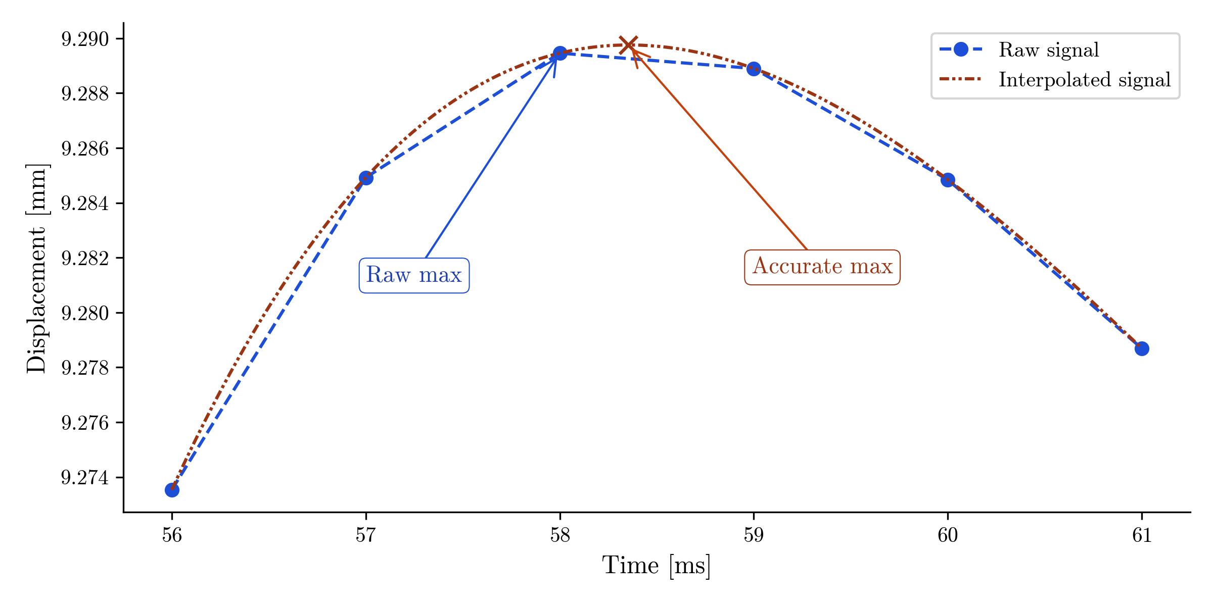
Plot showing zoomed-in portion of sampled TMG signal around its maximum, together with a polynonial interpolated through the maximum; the polynomial captures the true point of maximum muscle displacement, which falls between samples of the TMG signal.

You can solve this problem in practice by interpolating a polynomial around the peak of the TMG signal and computing the polynomial's maximum value.

Do you even need to interpolate?

The error in locating the maximum's time by taking the maximum sample in the raw signal is on the order of half the spacing between samples. Whether this is meaningful or not depends on the application—for a typical TMG signal sampled at 1 kHz (1 sample per millisecond), the error works out to something on the order of 0.5 ms. Typical values of Td and Tc can fall in the 15-25 milliseconds, where +/- 0.5 ms is enough to make a difference at the precision desired for TMG measurements, so we prefer to find the "true" maximum by interpolation.

For other applications the accuracy gained is insignificant, and you would prefer to avoid the extra computation involved.

Here is minimal working code:

For real-world code that handles edge cases and other real-world considerations, see [GitHub]

python

import numpy as np
from scipy.interpolate import lagrange

def interpolate_max(t, y):
    """ 
    Uses interpolation to estimate the "true" maximum of the discrete signal `y`.
    Returns a (t_max, y_max) tuple with the time and value of the interpolated
    maximum.

    Parameters
    ----------
    t : ndarray
        1D Numpy array of time points at which `y` is sampled.
    y : ndarray
        1D Numpy array containing signal whose maximum to interpolate.

    Returns
    ----------
    max : tuple
        Tuple (t_max, y_max) with time and value of interpolated maximum.

    (This is proof-of-concept, NOT real-world code. There is minimal bounds
    checking and handling of edge cases.)
    """
    
    # Maximum of sampled signal gives a rough idea of true maximum
    max_idx = np.argmax(y)

    # Generate a small window around maximum
    window_len = 2  # two points left of max, two points to the right
    t_window = []
    y_window = []
    for i in range(max_idx - window_len, max_idx + window_len + 1):
      if i >= 0 and i < len(y):  # stay in bounds
        t_window.append(i)
        y_window.append(y[i])

    # np.poly1d instance of polynomial interpolated through maximum
    poly = lagrange(t_window, y_window)

    # Evaluate polynomial on a finely spaced grid.
    # The interpolating polynomial's extremum is not found analytically, even #
    # though this is in principle possible. The extra precision is irrelevant and #
    # probably meaningless noise since the interpolation is an estimate anyway.
    magnification = 100  # e.g. 100 times more granular than sampling of `y`
    t_interp = np.linspace(t_window[0], t_window[-1], len(t_window)*magnification)
    y_interp = poly(t_interp)
    max_idx_interp = np.argmax(y_interp)
    return (t_interp[max_idx_interp], y_interp[max_idx_interp])

Other real-world considerations: distinguishing fast-twich and slow-twitch fibers

In practice, a TMG signal can have multiple local maxima during the contraction phase. When this occurs, it looks something like this:

[Graph of two-maxima TMG signal]

The contraction of fast-twitch fibers produces the first, smaller maximum, while slow-twitch fibers produce the second, larger maximum. Assuming one is using TMG for training/assessing speed and power, the first maximum should be used as a reference for time parameters.

But you also can't naively "take the first local maximum" in the TMG signal, because small artefacts from IIR filtering in the data acquisition pipeline produce maxima over the first few milliseconds of the TMG signal. In practice, a simple heuristic of ignoring maxima with a time less than a few milliseconds and contraction amplitude less than a few tenths of a millimeter effectively removes any false flags from IIR filter artefacts.

[Graph of IIR filter artefact]

For example, the source code for the function responsible for computing Dm includes the following parameters:

import numpy as np
from scipy.signal import find_peaks

def find_max(t, y, ignore_maxima_with_idx_less_than, ignore_maxima_less_than, use_first_max_as_dm, interpolate_dm):
    """
    Finds physiologically meaningful maximum contraction amplitude of TMG signal

    ignore_maxima_with_idx_less_than : int, optional
        Ignore data points with index less than
        `ignore_maxima_with_idx_less_than` when computing Dm. Used in practice
        to avoid tiny maxima resulting from filtering artefacts in the first
        few milliseconds of a TMG signal. Will use a sane default value
        designed for TMG signals if no value is specified.
    ignore_maxima_less_than : float, optional
        Ignore data points with values less than `ignore_maxima_less_than` when
        computing Dm. Used in practice to avoid tiny maxima resulting from
        filtering artefacts in the first few milliseconds of a TMG signal. Will
        use a sane default value designed for TMG signals if no value is
        specified.
    use_first_max_as_dm : bool
        If True, uses the first maximum meeting the criteria imposed by
        `ignore_maxima_with_idx_less_than` and `ignore_maxima_less_than` for
        Dm; if false, uses the global maximum for Dm. Used in practice to make
        Dm, and TMG parameters derived from it, correspond to the twitch from
        fast-twitch muscle fibers, which may have a distinct, earlier maximum
        than the global maximum caused by slower-twitch fibers.
    interpolate_dm : bool
        If True, uses interpolation to fine-tune the value of Dm beyond the
        granularity of `y`'s discrete samples. If False, uses the maximum
        sample in `y` as Dm. See `interpolate_max` for more context on
        interpolation.
    """
    # Finds all local maxima of sufficient height 
    max_idxs = find_peaks(y, height=ignore_maxima_less_than)[0]

    # Keep only maxima after ignore_maxima_with_idx_less_than
    max_idxs = max_idxs[(max_idxs > ignore_maxima_with_idx_less_than)]

    max_idx = int(max_idxs[0])  # cast is from np.int64 to int
    if not use_first_max_as_dm:
        for candidate in max_idxs:
            if y[candidate] > y[max_idx]:
                max_idx = candidate
    max_val = y[max_idx]

Takeaway: at this point we have the (interpolated) index and value of the maximum of the TMG signal. We then use the maximum value as a reference for computing time-based parameters.

Technique 2: Interpolating time of a target amplitude

[Recall overview]

The next step is to find the time at which the TMG signal:

first upcrosses above 10% max
first upcrosses above 50% max
first upcrosses above 90% max
first downcrosses below 90% max
first downcrosses below 50% max

Computationally, the problem here is to find the time at which a discrete, sampled signal passes through a target amplitude. Again we run into the problem of discrete sampling—in general the target amplitude will fall between points at which the signal was sampled, as shown in the graph below:

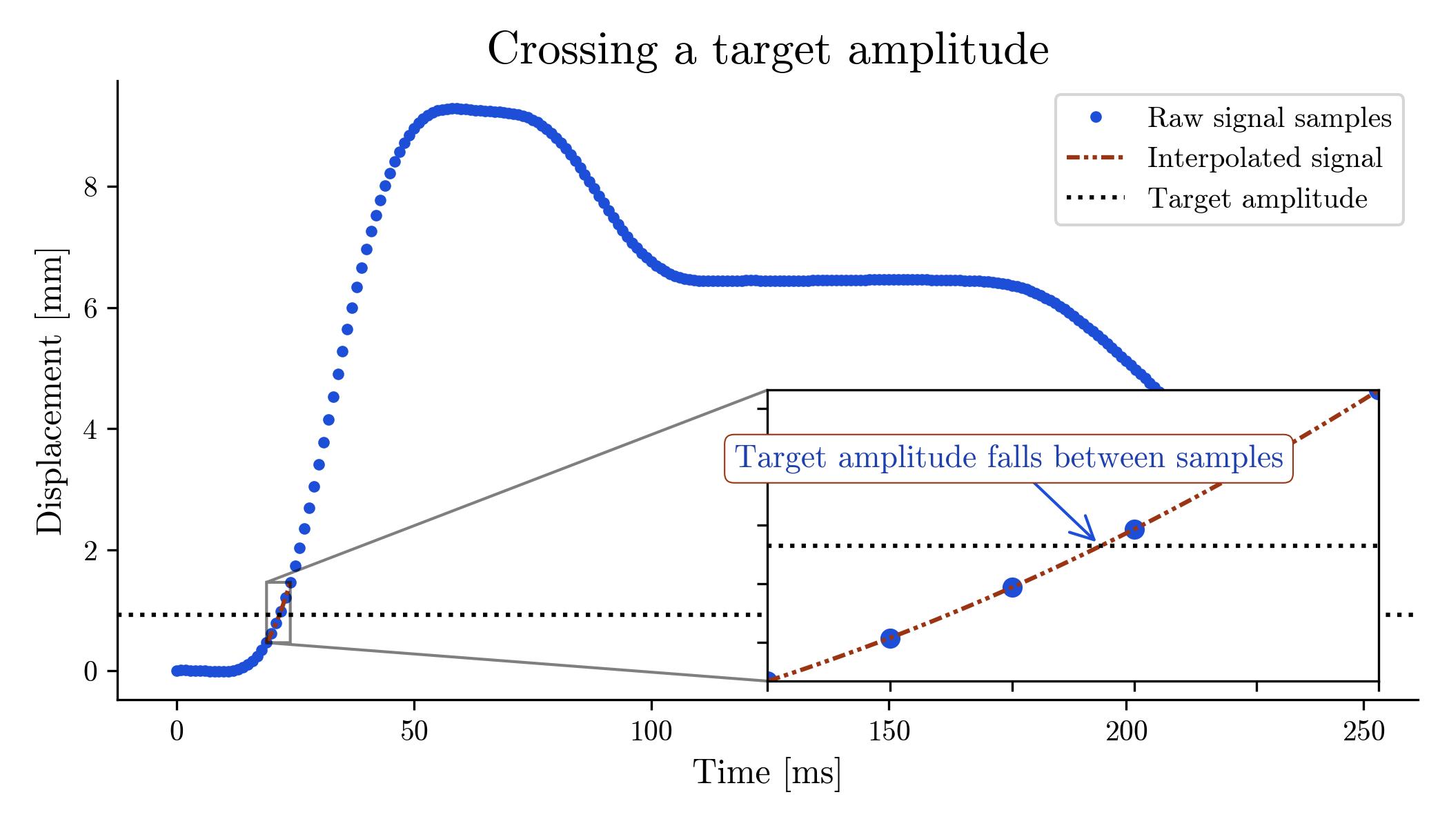
Target amplitude falls between TMG samples

We again solve this problem by using interpolation estimate the time at which the discrete sampled signal reaches a target amplitude with finer granularity than the signal's underlying sampling allows.

Concretely, we interpolate a Lagrange polynomial through the point of target amplitude, then uses a root-finding algorithm to find the time at which the interpolating polynomial crosses the target amplitude.

python

def _interpolate_idx_of_target_amplitude(y, target, upcrossing, start_search_at_idx=0):
  """Estimate index at which a time series reaches target amplitude.

    Uses interpolation to estimate the "index" at which a time series first
    reaches a target amplitude with finer granularity than the time series'
    underlying sampling allows.

    Used in practice to estimate the time when a TMG signal *first* reaches an
    amplitude equal to a target percentage of Dm (e.g. 10%, 50%, 90% etc.);
    this is nontrivial because generally the target amplitude falls between
    samples of the TMG signal, and so must be interpolated.

    The function interpolates a Lagrange polynomial around the point of target
    amplitude, then uses a root-finding algorithm to find the "index" value
    where the interpolating polynomial crosses the target amplitude.

    Note: 
    The function returns the estimated "index" at which the inputted signal
    would *first* reach the target amplitude if the signal were continuous.

    Parameters
    ----------
    y : ndarray
        1D Numpy array, in practice holding a TMG signal.
    target : double
        Target amplitude to find the index of.
    upcrossing : bool
        Set to `True` to find index at which `y` first crosses above `target`;
        set to `False` to find index at which `y` first crosses below `target`.
    start_search_at_idx : int, optional
        Only begin searching for target amplitude from this index onward.

    Returns
    ----------
    idx : float
        Estimated index at which `y` first reaches `target` amplitude.

    """
  # Find the two points enclosing target amplitude
  left_idx = None
  right_idx = None
  for i in range(start_search_at_idx, len(y) - 1):
    if upcrossing:
      if y[i] <= target and y[i + 1] >= target:
        left_idx = i
        right_idx = i + 1
        break
      else:
        if y[i] >= target and y[i + 1] <= target:
          left_idx = i
          right_idx = i + 1
          break

    if left_idx is None or right_idx is None:
      print("Error: no maximum found!", file=sys.stderr)
      sys.exit(1)

    # Store index of point closest to target amplitude.
    # (Used with root-finding algorithm below.)
    closest_idx_to_target = left_idx if abs(target - y[left_idx]) < abs(target - y[right_idx]) else right_idx

    # Create a window around target amplitude (as bounds permit)
    idx_window = []
    y_window = []
    window_len = 2  # two points left of max, two points to the right
    for i in range(left_idx - window_len, right_idx + window_len + 1):
      if i >= 0 and i < len(y):
        idx_window.append(i)
        y_window.append(y[i])

    # np.poly1d instance of polynomial interpolated through maximum
    poly = lagrange(t_window, y_window)
    coef = poly.coef

    # Subtract off target amplitude to prepare polynomial for use with a
    # root-finding algorithm
    coef[-1] -= target  

    # Points where interpolating polynomial equals target amplitude; cast to
    # real removes residual imaginary part left by the root-finding algorithm.
    roots = np.real(np.roots(coef))

    # The polynmial could in general have multiple roots; return the closest
    # root to the index of the target amplitude.
    return roots[np.argmin(np.abs(roots - closest_idx_to_target))]

Takeaway:

python

t10_upcross_idx = _interpolate_idx_of_target_amplitude(y, 0.1*dm, True)
t50_upcross_idx = _interpolate_idx_of_target_amplitude(y, 0.5*dm, True)
t90_upcross_idx = _interpolate_idx_of_target_amplitude(y, 0.9*dm, True)
t90_downcross_idx = _interpolate_idx_of_target_amplitude(y, 0.9*dm, False, start_search_at_idx=dm_idx)
t50_downcross_idx = _interpolate_idx_of_target_amplitude(y, 0.5*dm, False, start_search_at_idx=dm_idx)

Technique 3: Convert indices to times

Simple! But important.

Analysis of discrete signals works primarily in terms of indices into arrays. You need to convert these indices back to time to get human-facing results.

Compute time parameters:

python

# Convert indices to time
tm = _idx_to_time(float_dm_idx, t)
t10_upcross = _idx_to_time(t10_upcross_idx, t)
t50_upcross = _idx_to_time(t50_upcross_idx, t)
t90_upcross = _idx_to_time(t90_upcross_idx, t)
t90_downcross = _idx_to_time(t90_downcross_idx, t)
t50_downcross = _idx_to_time(t50_downcross_idx, t)


def _idx_to_time(idx, t):
  """Convert floating-point "index" to time value.

    Converts a (in-general) non-integer "index" into a time array into the
    units of the time. Used in practice after interpolating a TMG signal
    produces points that fall between discrete samples in the signal.

    Parameters
    ----------
    idx : float
        In-general floating-point index into `t`.
    t : ndarray
        1D array of time (or other independent variable) values.

    Returns
    ----------
    time : float
        Approximate independent variable value, in units of `t`, corresponding
        to `idx`; loosely, an estimate of the value t(idx) if `t` were
        continuous.
    """
  assert 0 <= idx < t.shape[0], "Index {} is out of bounds for time array with shape {}.".format(idx, t.shape)

  if idx.is_integer():
    return float(t[int(idx)])

    idx_floor = math.floor(idx)
    idx_ceil = math.ceil(idx)
    ratio = (idx - idx_floor)/(idx_ceil - idx_floor)

    t_floor = t[idx_floor]
    t_ceil = t[idx_ceil]
    return t_floor + ratio * (t_ceil - t_floor)

And compute TMG parameters:

python

# Compute standard TMG time parameters
td = t10_upcross
tc = t90_upcross - t10_upcross
ts = t50_downcross - t50_upcross
tr = t50_downcross - t90_downcross

TMG measurement computation algorithm

Here is the high-level process to computing the five TMG parameters:

Interpolate value and index of maximum amplitude
Interpolate the indices at which the TMG signal:
- first upcrosses above 10% max
- first upcrosses above 50% max
- first upcrosses above 90% max
- first downcrosses below 90% max
- first downcrosses below 50% max
Convert indices to times
Compute time parameters:

python

td = t10_upcross
tc = t90_upcross - t10_upcross
ts = t50_downcross - t50_upcross
tr = t50_downcross - t90_downcross

Convert indices to times

Compute time parameters:

python

# Convert indices to time
tm = _idx_to_time(float_dm_idx, t)
t10_upcross = _idx_to_time(t10_upcross_idx, t)
t50_upcross = _idx_to_time(t50_upcross_idx, t)
t90_upcross = _idx_to_time(t90_upcross_idx, t)
t90_downcross = _idx_to_time(t90_downcross_idx, t)
t50_downcross = _idx_to_time(t50_downcross_idx, t)


def _idx_to_time(idx, t):
  """Convert floating-point "index" to time value.

    Converts a (in-general) non-integer "index" into a time array into the
    units of the time. Used in practice after interpolating a TMG signal
    produces points that fall between discrete samples in the signal.

    Parameters
    ----------
    idx : float
        In-general floating-point index into `t`.
    t : ndarray
        1D array of time (or other independent variable) values.

    Returns
    ----------
    time : float
        Approximate independent variable value, in units of `t`, corresponding
        to `idx`; loosely, an estimate of the value t(idx) if `t` were
        continuous.
    """
  assert 0 <= idx < t.shape[0], "Index {} is out of bounds for time array with shape {}.".format(idx, t.shape)

  if idx.is_integer():
    return float(t[int(idx)])

    idx_floor = math.floor(idx)
    idx_ceil = math.ceil(idx)
    ratio = (idx - idx_floor)/(idx_ceil - idx_floor)

    t_floor = t[idx_floor]
    t_ceil = t[idx_ceil]
    return t_floor + ratio * (t_ceil - t_floor)

And compute TMG parameters:

python

# Compute standard TMG time parameters
td = t10_upcross
tc = t90_upcross - t10_upcross
ts = t50_downcross - t50_upcross
tr = t50_downcross - t90_downcross

Done!

TMG parameter computation ​

Synopsis ​

Problem statement ​

Technique 1: Interpolating maximum of a discrete signal ​

Other real-world considerations: distinguishing fast-twich and slow-twitch fibers ​

Technique 2: Interpolating time of a target amplitude ​

Technique 3: Convert indices to times ​

TMG measurement computation algorithm ​

Convert indices to times ​

TMG parameter computation

Synopsis

Problem statement

Technique 1: Interpolating maximum of a discrete signal

Other real-world considerations: distinguishing fast-twich and slow-twitch fibers

Technique 2: Interpolating time of a target amplitude

Technique 3: Convert indices to times

TMG measurement computation algorithm

Convert indices to times